Use Case For Wind Turbine Model: Example of "Application-As-a-Service"
Abstract
This article is to provide an idea of how to leverage DOME/DMC core assets to develop applications that can be shared with the connected community. The design/architecture of the application is very simplified in this example but it shows how one can use a Matlab Simulink model and share the results of the model with several end users. This is a good example for "Application-As-a-Service" and we show how this can analyze, automate and support business processes.
Introduction
This example of a Wind Model is done to demonstrate how we can use DOME and DMC to create useful applications. The set of technologies in this use case are the DOME Server, Dome Client, Visualization and we show how all these can be used for reducing product development times, cost and faster response to the market. Together with the technologies described above this use case includes engineering, process planning, simulation and decision making. We have not used any manufacturer-specific models of wind turbines and each of these models includes representations of general turbine aerodynamics, the mechanical drive-train, and the electrical characteristics of the generator and converter, as well as the control systems typically used. The models (doubly-fed induction generator model) have been used in this use case [1] [2].
Figure 1 shows the conceptual/technology stack in this application.
Figure 1: Technology stack for Wind Model
Description of the Wind Model
The blocks shown in Figure 2 is a simplified version of the Simulink Model shown in Figure 3. This represents a wind farm consisting of several wind turbines. In the Simulink model we have six 1.5 MW wind turbines connected to a 25 kV distribution system and exports power to a 120 kV grid through a 30 km, 25 kV feeder. Wind turbines using a doubly-fed induction generator (DFIG) consist of a wound rotor induction generator and an AC/DC/AC IGBT-based PWM converter. The stator winding is connected directly to the 60 Hz grid while the rotor is fed at variable frequency through the AC/DC/AC converter. The DFIG technology allows extracting maximum energy from the wind for low wind speeds by optimizing the turbine speed, while minimizing mechanical stresses on the turbine during gusts of wind.

Figure 2: Block Diagram
Figure 3 shown below is the actual Simulink Model where we have used the phasor model (continuous) because it is better adapted to simulate the low frequency electromechanical oscillations over long periods of time (tens of seconds to minutes). In the phasor simulation method, the sinusoidal voltages and currents are replaced by phasor quantities (complex numbers) at the system nominal frequency (50 Hz or 60 Hz).This is the same technique which is used in transient stability software. Each of the blocks in the model consist of several parameters. The parameters exposed for this use case are described below in Table 1.

Figure 3: Simulink Model
Use Case actors
Figure 4 illustrates at a very broad level the tasks performed by the Dome/DMC Developer so that the actors like Power System Planner, Power System Operator, Researcher, Consultant or Wind Plant developer can benefit by this application.We discuss each of the tasks shown here.

Figure 4: Use case Actors
Designing Wind Model Plugin
We started with the Simulink model shown in Figure 3, and decided on the parameters that can be changed by the actors who will use this appliction. Our goal was to do the simulations ahead of time for all the permutations of the changeable parameters so that the Dome Client can use the Simulated results. One could have saved the simulated results from Matlab Simulink in a databse but we have saved the simulink results in a mat file (power_wind_dfig_object_dome.mat) . The Dome Matlab Plugin is leveraged to extract output parameters .
Table 1 shows which parameters can be changed. Changing the parameter can affect one or more blocks in the Simulink model and we show that relationship in Table 1.
| Input Parameters | Variations | Applies to which blocks ( See Figure 2 above) |
|---|---|---|
| Frequency | 50 and 60 : Hz | 1,3,4,5,9 |
Number of Turbines | 2,3,4,5 and 6 | 6 |
| Starting Wind Speed | 4,5,6,7,8: m/s | 8 |
| Line Length | 10,50100: km | 4 |
Table 1: Simulink Model exposes these changeable Parameters
Table 2 shows output parameters from the Wind Model.
| Output Parameters | Description |
|---|---|
| Grid Data | The Simulink Scope with title "Data Acquisition" shown in Green color in figure 2. We see 8 plots |
| Wind Turbine Data | The Simulink Scope with title "Wind Turbine" shown in Green color in figure 2. We see 8 plots |
| Object Number | This is the object number in the mat file. Used for debugging purposes |
| Graph Titles | This is a text file that we upload with the titles for each of the plots. Useful when we plot the data in the Web Interface. |
Table 2: Ouput Parameters From Wind Model
Note that the Simulations were done for all the variations shown in Table 1 and we have output for 150 simulations. The object number shown in table 2 reflects the simulation output in the mat file (power_wind_dfig_object_dome.mat).
The motivation for the variations used in Table 1 was simply the design of the Dome Developer.
Figure 5 shows the development of the power_wind_dfig_object_dome.mat.
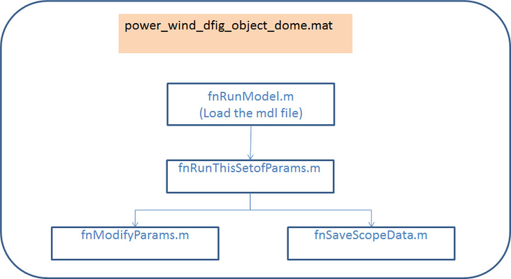
Figure 5: Development of the Wind Model Plugin
The code for the Simulink model and all the scripts are in this Dome_Wind_Model_Code.zip file. The contents of the zip file along with brief descriptions are as follows in Table 3.
| Matlab Script Name | Description |
|---|---|
fnRunModel.m | This script is run to so that we can save all the simulated objects in "power_wind_dfig_object_dome.mat". The Parameters that we allow the Dome Client to change must match the ones defined here |
| fnRunThisSetofParams.m | This runs the simulation and produces the plots in the Scopes defined in the Simulink model |
| fnModifyParms.m | This modifies the params in the blocks of the Simulink model before simulation can be run |
| fnSaveScopeData.m | The plots that are shown in the Scopes are saved so we can plot in Dome |
| power_wind_dfig.mdl | The Simulink model shown graphically in Figure 2. |
| power_wind_dfig_data.m | The initialization data needed by Simulink for this model |
Table 3: Description of Wind Model Matlab Files
Figure 6 shows a typical output from the Scopes of the Simulink Model.
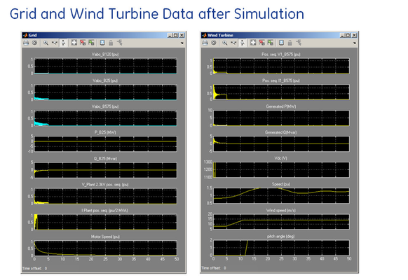
Figure 6: The data from the Scope of the Simulink Model
Figure 7 shows the matlab script for the Wind Model Plugin used in Dome
function [gD,tD,objNum] = fnGetWindDFIGData(iFreq, iLine,iNumT,iSpeed)
|
|---|
Figure 7: Wind Model Plugin - Matlab Script
Creating Dome Model
Please refer to "How to write third Party Models" where Matlab model is described. (/wiki/spaces/DMC/pages/21692467)
Shown below are screen shots for this Wind Model Use case.
- Figure 8 shows the Dome Model Build where we define the inputs and outputs
- Figure 9 shows the Dome Model Build where we define the causality
- Figure 10 shows the Dome Model Build where we define the setup
- Figure 11 shows the Dome Model Run where we select the Input parameters. Note since these were Enumerated types(Table 1- Values column) , while selecting in the drop down box, the values are shown in parenthesis, but after the selection is made it shows the Object id of the Enumerated parameter.
- Figure 12 shows the Dome Model Run after tDome has finished execution of the model. See that the Grid and Wind Turbine Matrix sizes have changed.
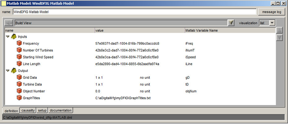
Figure 8: Dome Model Build - Input and Output
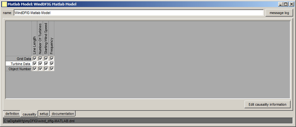
Figure 9: Dome Model Build - Causality
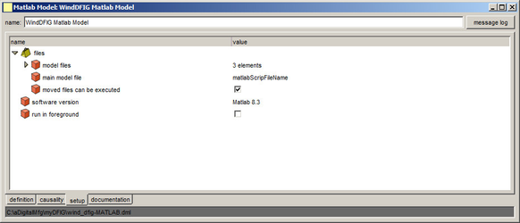
Figure 10: Dome Model Build - Setup
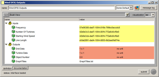
Figure 11: Dome Model Run - Selecting Inputs
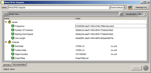
Figure 12: Dome Model Run - After execution
Developing Gaps that were not in DOME/DMC
It is quite possible that the existing code base in Dome/DMC may not exist for the application one is building. In this case when we were running the Wind Model script (Figure 7) we found that the matlab engine took longer time to load the mat file. So we had to modify the MatlabPluginR2014.dll. We added extra time for evaluation of the matlab engine command. Also if the matlab command in the script is long command then additional time was provided for its completion.
The Dome Model outputs shown in Figure 12 had to be plotted like how the Scope shows in Simulink. We did not have a charting tool to show multiple charts so we developed a servlet named "TwoColumnCharts". This servlet uses the titles from "GraphTitles.txt" (see table 2) and data from the Dome Model output. We do have an option to develop swing based java application and display the charts in Dome Client. This TwoColumnCharts servlet can be generalized but for now this serves this use case.
The servlet, TwoColumnCharts, in proxytest.html is as follows, where the param OutParamsData passes the data JsonText_2.txt as a text file. This text file data contains the data when ParameterValueChangeEvent occurs for the param name "Grid Data" and param name " Turbine Data". These were currently copied from from DomeApiServices.txt , but can be obtained by being a consumer to the ActiveMQ server queues.
<FORM METHOD="POST" ACTION="http://localhost:8080/SimpleServlet/TwoColumnCharts" >
<input type="hidden" name="OutParamsData" value="JsonText_2.txt"/>
<INPUT TYPE="SUBMIT" VALUE="TestServlet">
</FORM>
Visualization of the Wind Model Output plots
This use case was tested by first installing Tomacat Serve, ActiveMQ and DomeServicesAPIV7. Detailed instructions for setting this up is in /wiki/spaces/DMC/pages/19496967. We started Tomcat and ran /DomeApiServicesV7/proxytest.html. Figure 13 shows the result when the "Run" button was clicked for the "WindDFIG Matlab Model".
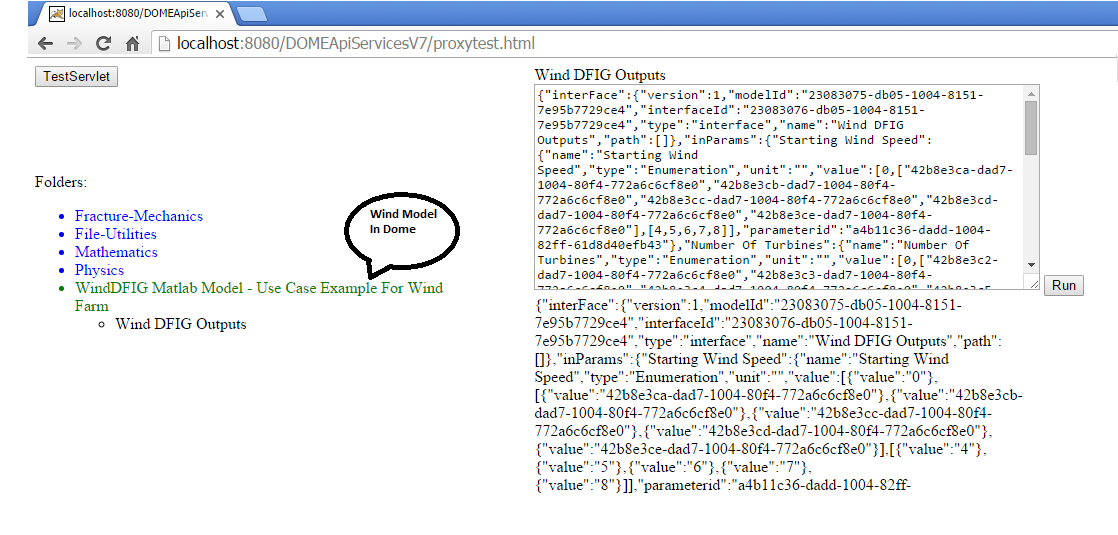
Figure 13: Wind Model run in the Web Browser
Notice that we added the button "TestServlet" in proxytest.html to test the TwoColumnCharts servlet. When we press that we get all the plots as shown below in Figure 14
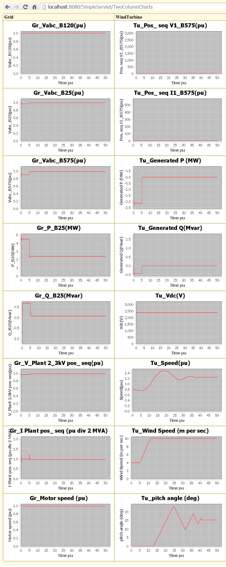
Figure 14: Plots from TwoColumnCharts Servlet
Conclusion
In this example we have shown how a Model Created in Matlab using Simulink is used by the user community to observe the behaviour of the Wind Turbine or Grid Data depending on the parameters selected by the user. This can be seen as a service to the user community who do not have the expensive Matlab Simulink. A researcher can analyze data,a power system planner can validate if Grid Data will meet reliability standards, Wind Plant developers can study the impact of the turbines, the operator can use the Grid Data and Turbine Data to troubleshoot when grid plots are not as expected and the Consultants can make proper business decisions like how many turnines to to order, location of the farm.
References
1] http://www.nrel.gov/docs/fy12osti/52780.pdf, National Renewable Energy Laboratory Report, Mohit Singh Surya Santoso.
2] http://www.mathworks.com/help/physmod/sps/examples/wind-farm-dfig-detailed-model.html, Richard Gagnon (Hydro-Quebec)